Examples
Load the PMF
From XLSX output
Given an output folder in /home/myname/Documents/PMF/GRE-cb/MobilAir_woOrga that looked like:
MobilAir_woOrga
├── GRE-cb_BaseErrorEstimationSummary.xlsx
├── GRE-cb_base.xlsx
├── GRE-cb_boot.xlsx
├── GRE-cb_ConstrainedDISPest.dat
├── GRE-cb_ConstrainedDISPres1.txt
├── GRE-cb_ConstrainedDISPres2.txt
├── GRE-cb_ConstrainedDISPres3.txt
├── GRE-cb_ConstrainedDISPres4.txt
├── GRE-cb_ConstrainedErrorEstimationSummary.xlsx
├── GRE-cb_Constrained.xlsx
├── GRE-cb_diagnostics.xlsx
├── GRE-cb_DISPest.dat
├── GRE-cb_DISPres1.txt
├── GRE-cb_DISPres2.txt
├── GRE-cb_DISPres3.txt
├── GRE-cb_DISPres4.txt
├── GRE-cb_Gcon_profile_boot.xlsx
├── GRE-cb_rotational_comments.txt
└── GRE-cb_sourcecontributions.xls
in order to convert them to a PMF object, run the following command :
from pyPMF.PMF import PMF

grecb = PMF(site="GRE-cb", reader="xlsx", BDIR="/home/myname/Documents/PMF/GRE-cb/MobilAir_woOrga")
From SQL database
It is also possible to load data from a SQL database. Here after is an example with a sqlite3 database, but as long as a proper connector is provided, it could be anything (MySQL, Postgres, etc.).
Default tables are :
Content |
Table name |
|---|---|
Base contributions |
PMF_dfcontrib_b |
Constrained contributions |
PMF_dfcontrib_c |
Base profiles |
PMF_dfprofiles_b |
Constrained profiles |
PMF_dfprofiles_c |
Base bootstrap |
PMF_dfBS_profile_b |
Constrained bootstrap |
PMF_dfBS_profile_c |
Base uncertainties summary |
PMF_df_uncertainties_summary_b |
Constrained uncertainties summary |
PMF_df_uncertainties_summary_c |
Base bootstrap mapping |
PMF_dfbootstrap_mapping_b |
Constrained bootstrap mapping |
PMF_dfbootstrap_mapping_c |
Base disp swap count |
PMF_df_disp_swap_b |
Constrained disp swap count |
PMF_df_disp_swap_c |
but you can provided custom table names from the SQL_tables_names argument.
import sqlite3
from pyPMF.PMF import PMF

conn = sqlite3.connect("./DB_PMF.db")

grecb = PMF(site="GRE-cb", reader="sql", SQL_connection=conn)

conn.close()
PMF object
Either way, now, grecb is an instance of a PMF object, and has read and plot abilities.
Read the data
Organization
The read class of the PMF object give access to different reader to retreive data from
the different data outputed by the EPA PMF5 software.
They all start by read_base* or read_constrained* name, for the base and constrained
run, respectively.
The special method read_metadata is used to retrieve the factors names and species names
from the base run, and use them everywhere else. It also try to set the total
variable name if any (one of PM10, PM2.5, PMrecons, PM10rec, PM10recons, otherwise try to
guess), used to convert unit and to be the default variable to plot.
For now, the following readers are implemented :
read.read_metadata
read.read_base_contributions : Contribution
read.read_base_profiles : Chemical profiles
read.read_base_bootstrap : All bootstrap profiles
read.read_base_uncertainties_summary : Summary
read.read_constrained_contributions : Contribution
read.read_constrained_profiles : Chemical profiles
read.read_constrained_bootstrap : All bootstrap profiles
read.read_constrained_uncertainties_summary : Summary
read.read_all
Contribution
The contributions of the factors (G matrix) are read from the _base.xlsx and
_Constrained.xlsx files, sheet contributions.
You can read them using the reader read_base_contributions and
read_constrained_contributions:
grecb.read.read_base_contributions()
grecb.read.read_constrained_contributions()
And now, the grecb object has a dfcontrib_b and dfcontrib_c attributes (_b for the
base run, _c for the constrained run):
>>> grecb.dfcontrib_c

            Sulfate-rich  Nitrate-rich  ...  Biomass burning  Sea/road salt  Mineral dust
Date                                    ...
2017-02-28      0.321580     -0.105980  ...          0.19419       0.606290      0.182880
2017-03-03      0.429480     -0.038802  ...          0.61595       0.050129      0.382890
2017-03-06     -0.098123     -0.151530  ...          0.53346       4.636400      0.272410
2017-03-09      0.643500     -0.002527  ...          1.09060       0.153200      1.083600
2017-03-12      0.664090      0.308390  ...          1.70740      -0.200000      0.846930
which is the G matrix, in normalized unit.
Chemical profiles
The chemical profiles (or simply profiles) is the F matrix of the PMF (in µg/m³) and
are read from the _base.xslx and _Constrained.xlsx files, sheet Profiles.
You can read them using the reader read_base_profiles and read_constrained_profiles:
grecb.read.read_base_profile()
grecb.read.read_constrained_profile()
and grecb has now dfprofiles_b and dfprofiles_c dataframe :
>>> grecb.dfprofiles_c
              Sulfate-rich  Nitrate-rich  ...  Biomass burning  Sea/road salt  Mineral dust
specie                                    ...
PMrecons          4.402500      2.421300  ...         3.027900       0.364280      2.009600
OC*               1.225300      0.000000  ...         1.308900       0.041038      0.428110
EC                0.162970      0.000000  ...         0.347050       0.019199      0.030703
Cl-               0.000000      0.002425  ...         0.026819       0.109070      0.000000
NO3-              0.300660      1.702200  ...         0.093396       0.000000      0.000000
SO42-             0.977680      0.010441  ...         0.092800       0.032969      0.189890
...                    ...           ...  ...             ...            ...           ...
The values are in µg/m³.
Uncertainties
Summary
You can also read the bootstrap and DISP results from the
_BaseErrorEstimationSummary.xlsx and _ConstrainedErrorEstimationSummary.xlsx files.
grecb.read.read_base_summary()
grecb.read.read_constrained_summary()
and now, you have access to df_uncertainties_summary_b and df_uncertainties_summary_c:
the summaries of the BS, DISP and BS-DISP uncertainties for each profiles and species.
>>> grecb.df_uncertainties_summary_c
                       Constrained base run    BS 5th  BS median   BS 95th  BS-DISP 5th  BS-DISP average  BS-DISP 95th  DISP Min  DISP average  DISP Max
profile      specie
Sulfate-rich PMrecons              4.402500  4.261867   4.511374  4.709612          NaN              NaN           NaN  3.788500      4.337850  4.887200
             OC*                   1.225300  0.822712   1.161025  1.702325          NaN              NaN           NaN  0.988480      1.211690  1.434900
             EC                    0.162970  0.051262   0.211147  0.436615          NaN              NaN           NaN  0.121070      0.213030  0.304990
             Cl-                   0.000000  0.000000   0.000000  0.000000          NaN              NaN           NaN  0.000000      0.006156  0.012311
             NO3-                  0.300660  0.000000   0.346984  0.563892          NaN              NaN           NaN  0.068862      0.260436  0.452010
...                                     ...       ...        ...       ...          ...              ...           ...       ...           ...       ...
Mineral dust Se                    0.000008  0.000000   0.000012  0.000029          NaN              NaN           NaN  0.000000      0.000023  0.000046
             Sn                    0.000000  0.000000   0.000032  0.000154          NaN              NaN           NaN  0.000000      0.000069  0.000139
             Ti                    0.002545  0.001121   0.001750  0.002546          NaN              NaN           NaN  0.002881      0.003464  0.004047
             V                     0.000265  0.000063   0.000145  0.000249          NaN              NaN           NaN  0.000265      0.000278  0.000290
             Zn                    0.000218  0.000000   0.000030  0.001286          NaN              NaN           NaN  0.000000      0.000177  0.000354
All bootstrap profiles
If you want to retreive the individual bootstrap results, read from
_boot.xlsx and _Gcon_profile_boot.xlsx:
grecb.read.read_base_bootstrap()
grecb.read.read_constrained_bootstrap()
and now you have access to dfBS_profile_b and dfBS_profile_c, which are all the
bootstrap chemical profiles for the base and constrained run, respectively.
>>> grecb.dfBS_profile_c
                              Boot0     Boot1     Boot2  ...    Boot97    Boot98   Boot100
specie   profile                                         ...
PMrecons Sulfate-rich      4.412330  2.259480  4.330630  ...  3.191810  4.041220  3.109190
         Nitrate-rich      2.462740  2.254470  2.609910  ...  2.068200  2.349640  2.404520
         Industrial        0.259120  0.289952  0.474484  ...  0.214298  0.206250  0.875102
         Primary biogenic  0.579702  1.437820  0.633064  ...  1.290640  0.358833  0.296207
         Primary traffic   1.862990  1.178150  1.711440  ...  1.171830  1.974060  1.678320
...                             ...       ...       ...  ...       ...       ...       ...
Zn       Marine SOA        0.000826  0.002239  0.001256  ...  0.000265  0.000389  0.000436
         Aged seasalt      0.000000  0.000000  0.000000  ...  0.000814  0.000304  0.001018
         Biomass burning   0.002404  0.001699  0.002053  ...  0.002012  0.002270  0.001188
         Sea/road salt     0.000625  0.000457  0.000848  ...  0.000234  0.000596  0.000187
         Mineral dust      0.000000  0.000000  0.000000  ...  0.001355  0.000000  0.000000
as well as dfbootstrap_mapping_b and dfbootstrap_mapping_c, which are the
tables of the mapping between reference and BS factors:
>>> grecb.dfbootstrap_mapping_c
                    Sulfate-rich Nitrate-rich Industrial Primary biogenic Primary traffic Marine SOA Aged seasalt Biomass burning Sea/road salt Mineral dust unmapped
BF-Sulfate-rich               94            0          2                0               3          0            0               0             0            0        0
BF-Nitrate-rich                0           99          0                0               0          0            0               0             0            0        0
BF-Industrial                  0            0         99                0               0          0            0               0             0            0        0
BF-Primary biogenic            0            0          0               99               0          0            0               0             0            0        0
BF-Primary traffic             0            0          0                0              99          0            0               0             0            0        0
BF-Marine SOA                  0            0          0                0               1         98            0               0             0            0        0
BF-Aged seasalt                0            0          0                0               0          0           99               0             0            0        0
BF-Biomass burning             0            0          0                0               0          0            0              99             0            0        0
BF-Sea/road salt               0            0          0                0               0          0            0               0            99            0        0
BF-Mineral dust                0            0          0                0               0          0            0               0             0           99        0
Plot utilities
For now, the following plotters are implemented :
plot.plot_per_microgramm : Chemical profile (per microgram of total variable)
plot.plot_totalspeciesum : Chemical profile (in percentage of the sum of each species)
plot.plot_stacked_profiles : Chemical profile stacked (in percentage of the sum of each species)
plot.plot_contrib : Contribution time series and uncertainties
plot.plot_all_profiles : Profiles plot summary
plot.plot_stacked_contribution : Stacked contributions
plot.plot_samples_sources_contribution : Stacked samples contributions
plot.plot_seasonal_contribution : Seasonnal contribution
plot.plot_polluted_contributions :
Chemical profile (per microgram of total variable)
grecb.plot.plot_per_microgramm(profiles=["Primary biogenic"])
Primary biogenic factor chemical profile as % of total variable.
Chemical profile (in percentage of the sum of each species)
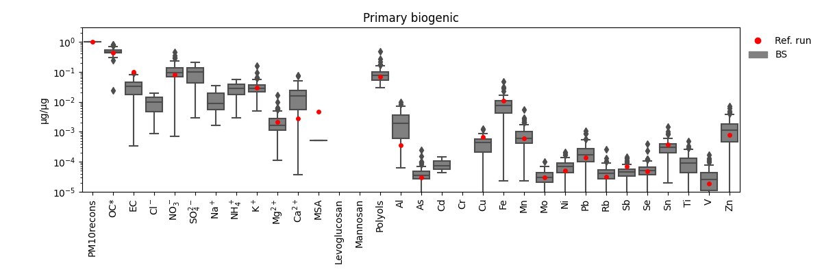
grecb.plot.plot_totalspeciesum(profiles=["Primary biogenic"])

Primary biogenic factor chemical profile as % of total specie sum.
Contribution time series and uncertainties
grecb.plot.plot_contrib(profiles=["Primary biogenic"])
will produce the following graph
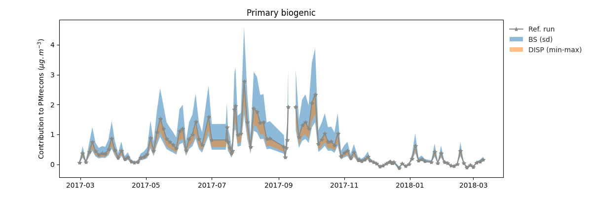
Primary biogenic factor total variable (i.e. PM10) contribution in µg/m³.
Since the EPA PMF5 does not output the chemical profile (F) matrix of the boostrap, the
uncertainties is estimated by computing the species concentration given the F matrix of
the reference run and the G matrix of the bootstrap run. As a result, the output is
“hacky” since in the bootstrap method, both the F and G matrix are changing. If you want
to remove them, just pass BS=False to the method.
Profiles plot summary
grecb.plot.plot_all_profiles(profiles=["Primary traffic"])
will produce the following graph

Primary traffic factor description.
Seasonnal contribution
grecb.plot.plot_seasonal_contribution(normalize=False, annual=False)
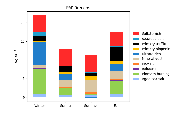
Seasonnal mean contribution of the factors to the PM mass.
Chemical profile stacked (in percentage of the sum of each species)
grecb.plot.plot_stacked_profiles()
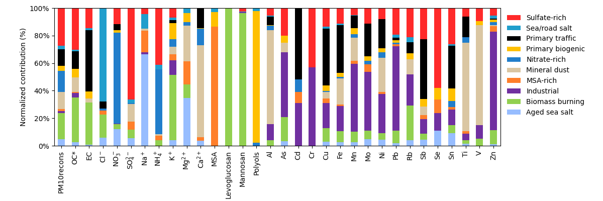
Contribution of each factor to the different species
Stacked contributions
grecb.plot.plot_stacked_contribution()
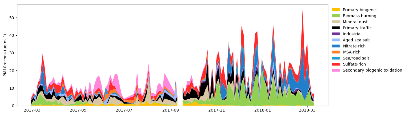
Stacked contribution timeseries to the PM mass.
Attention : This kind of graph is often misleading due to interpolation between days. Therefor, I recommand not to use it… Prefere the Stacked samples contributions one.
Stacked samples contributions
grecb.plot.plot_samples_sources_contribution()
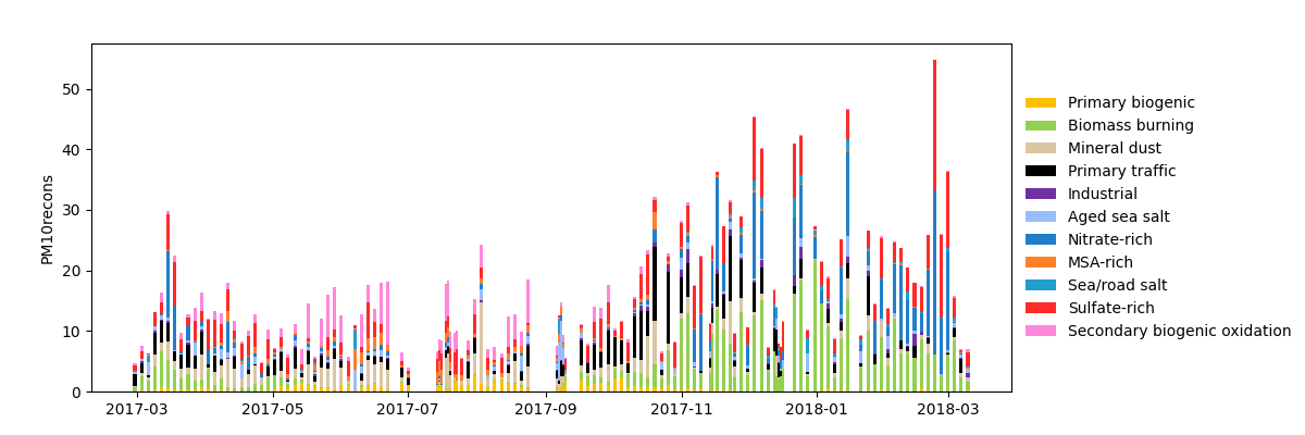
Stacked samples contribution timeseries to the PM mass.
By default, the width of a bar is 1.5 day. For sampling period lower than that, 1 day is used.
Utilities
Convert to cubic meter
In order to have the contributions in µg/m³, which is given by G⋅F, we need to know
both the chemical profile F and the contribution G.
And we can easily reconstruct the time serie in µg/m³ of each specie for every profile
by simple multiplication of the timeserie by the concentration in the chemical profile.
Since this is a very often computation, the method to_cubic_meter does just that :
>>> grecb.to_cubic_meter()
            Sulfate-rich  Nitrate-rich  ... Biomass burning  Sea/road salt  Mineral dust
Date                                    ...
2017-02-28      1.415756     -0.256609  ...        0.587988       0.220859      0.367516
2017-03-03      1.890786     -0.093951  ...        1.865035       0.018261      0.769456
2017-03-06     -0.431987     -0.366900  ...        1.615264       1.688948      0.547435
2017-03-09      2.833009     -0.006120  ...        3.302228       0.055808      2.177603
2017-03-12      2.923656      0.746705  ...        5.169836      -0.072856      1.701991
...                  ...           ...  ...             ...            ...           ...
Note that to_cubic_meter use by default the constrained run, all the profile
and the total variable, but you can specify other conditions (see [the doc of
this method](api.html#pyPMF.PMF.PMF.to_cubic_meter)).
Relative contributions of species to the total mass
By default, the profile matrix F is in µg/m³. But it’s often convenient to know the
relative contribution of each species to the “total variable” mass (for instance, percent of
contribution of each specie to the $PM_10$).
This result is the ratio of each species in a profile to the total variable.
The method to_relative_mass conveniently handle it, and return you a new dataframe:
>>> grecb.to_relative_mass()
              Sulfate-rich  Nitrate-rich  ... Biomass burning  Sea/road salt  Mineral dust
specie                                    ...
PMrecons          1.000000      1.000000  ...        1.000000       1.000000      1.000000
OC*               0.278319      0.000000  ...        0.432280       0.112655      0.213032
EC                0.037018      0.000000  ...        0.114617       0.052704      0.015278
Cl-               0.000000      0.001002  ...        0.008857       0.299413      0.000000
NO3-              0.068293      0.703011  ...        0.030845       0.000000      0.000000
SO42-             0.222074      0.004312  ...        0.030648       0.090505      0.094491
...                    ...           ...  ...             ...            ...           ...
The values are now in % of the PMrecons mass.
Relative contribution of the factor for each species
Another usefull information is how much a given specie is apportioned by all factors, denoted as the total specie sum graph in the EPA PMF5 software. It is the amount of a given specie in a factor divided by the sum of this specie in all factors.
The method get_total_specie_sum return this value for every species in all profiles:
>>> grecb.get_total_specie_sum()
              Sulfate-rich  Nitrate-rich  ...  Biomass burning  Sea/road salt  Mineral dust
specie                                    ...
PMrecons         27.520080     15.135575  ...        18.927439       2.277119     12.562033
OC*              30.440474      0.000000  ...        32.517372       1.019519     10.635658
EC               14.525003      0.000000  ...        30.931475       1.711146      2.736462
Cl-               0.000000      1.506558  ...        16.659544      67.752580      0.000000
NO3-             11.676593     66.107550  ...         3.627177       0.000000      0.000000
SO42-            66.571611      0.710942  ...         6.318883       2.244906     12.929878
...                    ...           ...  ...             ...            ...           ...
In this example, the Biomass burning factor apportion 18% of the total PMrecons, 32% of the OC*, 30% of the EC, etc. We also see that the NO3- is mainly apportioned by the Nitrate-rich factor (66%).